On word embeddings - Part 2: Approximating the Softmax
The softmax layer is a core part of many current neural network architectures. When the number of output classes is very large, such as in the case of language modelling, computing the softmax becomes very expensive. This post explores approximations to make the computation more efficient.

This post gives an overview of approximations that can be used to make the expensive softmax layer more efficient.
Table of contents:
This is the second post in a series on word embeddings and representation learning. In the previous post, we gave an overview of word embedding models and introduced the classic neural language model by Bengio et al. (2003), the C&W model by Collobert and Weston (2008), and the word2vec model by Mikolov et al. (2013). We observed that mitigating the complexity of computing the final softmax layer has been one of the main challenges in devising better word embedding models, a commonality with machine translation (MT) (Jean et al., 2015) [1] and language modelling (Jozefowicz et al., 2016) [2].
In this post, we will thus focus on giving an overview of various approximations to the softmax layer that have been proposed over the last years, some of which have so far only been employed in the context of language modelling or MT. We will postpone the discussion of additional hyperparameters to the subsequent post.
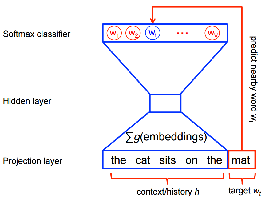
Let us know partially re-introduce the previous post's notation both for consistency and to facilitate comparison as well as introduce some new notation: We assume a training corpus containing a sequence of \(T\) training words \(w_1, w_2, w_3, \cdots, w_T\) that belong to a vocabulary \(V\) whose size is \(|V|\). Our models generally consider a context \(c\) of \( n \) words. We associate every word with an input embedding \( v_w \) (the eponymous word embedding in the Embedding Layer) with \(d\) dimensions and an output embedding \( v'_w \) (the representation of the word in the weight matrix of the softmax layer). We finally optimize an objective function \(J_\theta\) with regard to our model parameters \(\theta\).
Recall that the softmax calculates the probability of a word \(w\) given its context \(c\) and can be computed using the following equation:
\(p(w | c) = \dfrac{\text{exp}({h^\top v'_w})}{\sum_{w_i \in V} \text{exp}({h^\top v'_{w_i}})} \)
where \(h\) is the output vector of the penultimate network layer. Note that we use \(c\) for the context as mentioned above and drop the index \(t\) of the target word \(w_t\) for simplicity. Computing the softmax is expensive as the inner product between \(h\) and the output embedding of every word \(w_i\) in the vocabulary \(V\) needs to be computed as part of the sum in the denominator in order to obtain the normalized probability of the target word \(w\) given its context \(c\).
In the following we will discuss different strategies that have been proposed to approximate the softmax. These approaches can be grouped into softmax-based and sampling-based approaches. Softmax-based approaches are methods that keep the softmax layer intact, but modify its architecture to improve its efficiency. Sampling-based approaches on the other hand completely do away with the softmax layer and instead optimise some other loss function that approximates the softmax.
Softmax-based Approaches
Hierarchical Softmax
Hierarchical softmax (H-Softmax) is an approximation inspired by binary trees that was proposed by Morin and Bengio (2005) [3]. H-Softmax essentially replaces the flat softmax layer with a hierarchical layer that has the words as leaves, as can be seen in Figure 1.
This allows us to decompose calculating the probability of one word into a sequence of probability calculations, which saves us from having to calculate the expensive normalization over all words. Replacing a softmax layer with H-Softmax can yield speedups for word prediction tasks of at least \(50 \times\) and is thus critical for low-latency tasks such as real-time communication in Google's new messenger app Allo.

We can think of the regular softmax as a tree of depth \(1\), with each word in \(V\) as a leaf node. Computing the softmax probability of one word then requires normalizing over the probabilities of all \(|V|\) leaves. If we instead structure the softmax as a binary tree, with the words as leaf nodes, then we only need to follow the path to the leaf node of that word, without having to consider any of the other nodes.
Since a balanced binary tree has a depth of \(\text{log}_2 (|V|)\), we only need to evaluate at most \(\text{log}_2 (|V|)\) nodes to obtain the final probability of a word. Note that this probability is already normalized, as the probabilities of all leaves in a binary tree sum to \( 1 \) and thus form a probability distribution. To informally verify this, we can reason that at a tree's root node (Node 0) in Figure 1), the probabilities of branching decisions must sum to \(1\). At each subsequent node, the probability mass is then split among its children, until it eventually ends up at the leaf nodes, i.e. the words. Since no probability is lost along the way and since all words are leaves, the probabilities of all words must necessarily sum to \(1\) and hence the hierarchical softmax defines a normalized probability distribution over all words in \(V\).
To get a bit more concrete, as we go through the tree, we have to be able to calculate the probability of taking the left or right branch at every junction. For this reason, we assign a representation to every node. In contrast to the regular softmax, we thus no longer have output embeddings \(v'_w\) for every word \(w\) -- instead, we have embeddings \(v'_n\) for every node \(n\). As we have \(|V|-1\) nodes and each one possesses a unique representation, the number of parameters of H-Softmax is almost the same as for the regular softmax. We can now calculate the probability of going right (or left) at a given node \(n\) given the context \(c\) the following way:
\( p(\text{right} | n, c) = \sigma (h^\top v'_{n})\).
This is almost the same as the computations in the regular softmax; now instead of computing the dot product between \(h\) and the output word embedding \(v'_{w}\), we compute the dot product between \(h\) and the embedding \(v'_{w}\) of each node in the tree; additionally, instead of computing a probability distribution over the entire vocabulary words, we output just one probability, the probability of going right at node \(n\) in this case, with the sigmoid function. Conversely, the probability of turning left is simply \( 1 - p( \text{right} | n,c)\).

The probability of a word \(w\) given its context \(c\) is then simply the product of the probabilities of taking right and left turns respectively that lead to its leaf node. To illustrate this, given the context "the", "dog", "and", "the", the probability of the word "cat" in Figure 2 can be computed as the product of the probability of turning left at node 1, turning right at node 2, and turning right at node 5. Hugo Lachorelle gives a more detailed account in his excellent lecture video. Rong (2014) [4] also does a good job of explaining these concepts and also derives the derivatives of H-Softmax.
Obviously, the structure of the tree is of significance. Intuitively, we should be able to achieve better performance, if we make it easier for the model to learn the binary predictors at every node, e.g. by enabling it to assign similar probabilities to similar paths. Based on this idea, Morin and Bengio use the synsets in WordNet as clusters for the tree. However, they still report inferior performance to the regular softmax. Mnih and Hinton (2008) [5] learn the tree structure with a clustering algorithm that recursively partitions the words in two clusters and allows them to achieve the same performance as the regular softmax at a fraction of the computation.
Notably, we are only able to obtain this speed-up during training, when we know the word we want to predict (and consequently its path) in advance. During testing, when we need to find the most likely prediction, we still need to calculate the probability of all words, although narrowing down the choices in advance helps here.
In practice, instead of using "right" and "left" in order to designate nodes, we can index every node with a bit vector that corresponds to the path it takes to reach that node. In Figure 2, if we assume a 0 bit for turning left and a 1 bit for turning right, we can thus represent the path to "cat" as 011.
Recall that the path length in a balanced binary tree is \(\text{log}_2 |V|\). If we set \(|V| = 10000\), this amounts to an average path length of about \( 13.3 \). Analogously, we can represent every word by the bit vector of its path that is on average \(13.3\) bits long. In information theory, this is referred to as an information content of \(13.3\) bits per word.
A note on the information content of words
Recall that the information content \(I(w)\) of a word \(w\) is the negative logarithm of its probability \(p(w)\):
\(I(w) = -\log_2 p(w) \).
The entropy \( H \) of all words in a corpus is then the expectation of the information content of all words in the vocabulary:
\( H = \sum_{i\in V} p(w_i) I(w_i) \).
We can also conceive of the entropy of a data source as the average number of bits needed to encode it. For a fair coin flip, we need \(1\) bit per flip, whereas we need \(0\) bits for a data source that always emits the same symbol. For a balanced binary tree, where we treat every word equally, the word entropy \(H\) equals the information content \(I(w)\) of every word \(w\), as each word has the same probability. The average word entropy \(H\) in a balanced binary tree with \(|V| = 10000\) thus coincides with its average path length:
\( H = - \sum_{i\in V} \dfrac{1}{10000} \log_2 \dfrac{1}{10000} = 13.3\).
We saw before that the structure of the tree is important. Notably, we can leverage the tree structure not only to gain better performance, but also to speed up computation: If we manage to encode more information into the tree, we can get away with taking shorter paths for less informative words. Morin and Bengio point out that leveraging word probabilities should work even better; as some words are more likely to occur than others, they can be encoded using less information. They note that the word entropy of their corpus (with \(|V| = 10,000\)) is about \( 9.16 \).
Thus, by taking into account frequencies, we can reduce the average number of bits per word in the corpus from \( 13.3 \) to \( 9.16 \) in this case, which amounts to a speed-up of 31%. A Huffman tree, which is used by Mikolov et al. (2013) [6] for their hierarchical softmax, generates such a coding by assigning fewer bits to more common symbols. For instance, "the", the most common word in the English language, would be assigned the shortest bit code in the tree, the second most frequent word would be assigned the second-shortest bit code, and so on. While we still need the same number of codes to designate all words, when we predict the words in a corpus, short codes appear now a lot more often, and we consequently need fewer bits to represent each word on average.
A coding such as Huffman coding is also known as entropy encoding, as the length of each codeword is approximately proportional to the entropy of each symbol as we have observed. Shannon (1951) [7] establishes in his experiments that the lower bound on the information rate in English is between \(0.6\) to \(1.3\) bits per character; given an average word length of \(4.5\), this amounts to \(2.7\) - \(5.85\) bits per word.
To tie this back to language modelling (which we already talked about in the previous post): perplexity, the evaluation measure of language modelling, is \(2^{H}\) where \(H\) is the entropy. A unigram entropy of \( 9.16 \) thus entails a still very high perplexity of \( 2^{9.16} = 572.0\). We can render this value more tangible by observing that a model with a perplexity of \(572\) is as confused by the data as if it had to choose among \(572\) possibilities for each word uniformly and independently.
To put this into context: The state-of-the-art language model by Jozefowicz et al. (2016) achieves a perplexity of \(24.2\) per word on the 1B Word Benchmark. Such a model would thus require an average of around \(4.60\) bits to encode each word, as \( 2^{4.60} = 24.2 \), which is incredibly close to the experimental lower bounds documented by Shannon. If and how we could use such a model to construct a better hierarchical softmax layer is still left to be explored.
Differentiated Softmax
Chen et al. (2015) [8] introduce a variation on the traditional softmax layer, the Differentiated Softmax (D-Softmax). D-Softmax is based on the intuition that not all words require the same number of parameters: Many occurrences of frequent words allow us to fit many parameters to them, while extremely rare words might only allow to fit a few.
In order to do this, instead of the dense matrix of the regular softmax layer of size \(d \times |V| \) containing the output word embeddings \( v'_w \in \mathbb{R}^d \), they use a sparse matrix. They then arrange \( v'_w\) in blocks sorted by frequency, with the embeddings in each block being of a certain dimensionality \(d_k \). The number of blocks and their embedding sizes are hyperparameters that can be tuned.

In Figure 3, embeddings in partition \(A\) are of dimensionality \(d_A\) (these are embeddings of frequent words, as they are allocated more parameters), while embeddings in partitions \(B\) and \(C\) have \(d_B\) and \(d_C\) dimensions respectively. Note that all areas not part of any partition, i.e. the non-shaded areas in Figure 1, are set to \(0\).
The output of the previous hidden layer \(h\) is treated as a concatenation of features corresponding to each partition of the dimensionality of that partition, e.g. \(h\) in Figure 3 is made up of partitions of size \(d_A\), \(d_B\), and \(d_B\) respectively. Instead of computing the matrix-vector product between the entire output embedding matrix and \(h\) as in the regular softmax, D-Softmax then computes the product of each partition and its corresponding section in \(h\).
As many words will only require comparatively few parameters, the complexity of computing the softmax is reduced, which speeds up training. In contrast to H-Softmax, this speed-up persists during testing. Chen et al. (2015) observe that D-Softmax is the fastest method when testing, while being one of the most accurate. However, as it assigns fewer parameters to rare words, D-Softmax does a worse job at modelling them.
CNN-Softmax
Another modification to the traditional softmax layer is inspired by recent work by Kim et al. (2016) [9] who produce input word embeddings \(v_w\) via a character-level CNN. Jozefowicz et al. (2016) in turn suggest to do the same thing for the output word embeddings \(v'_w\) via a character-level CNN -- and refer to this as CNN-Softmax. Note that if we have a CNN at the input and at the output as in Figure 4, the CNN generating the output word embeddings \(v'_w\) is necessarily different from the CNN generating the input word embeddings \(v_w\), just as the input and output word embedding matrices would be different.

While this still requires computing the regular softmax normalization, this approach drastically reduces the number of parameters of the model: Instead of storing an embedding matrix of \(d \times |V| \), we now only need to keep track of the parameters of the CNN. During testing, the output word embeddings \(v'_w\) can be pre-computed, so that there is no loss in performance.
However, as characters are represented in a continuous space and as the resulting model tends to learn a smooth function mapping characters to a word embedding, character-based models often find it difficult to differentiate between similarly spelled words with different meanings. To mitigate this, the authors add a correction factor that is learned per word, which significantly reduces the performance gap between regular and CNN-softmax. By adjusting the dimensionality of the correction term, the authors are able to trade-off model size versus performance.
The authors also note that instead of using a CNN-softmax, the output of the previous layer \(h\) can be fed to a character-level LSTM, which predicts the output word one character at a time. Instead of a softmax over words, a softmax outputting a probability distribution over characters would thus be used at every time step. They, however, fail to achieve competitive performance with this layer. Ling et al. (2016) [10] use a similar layer for machine translation and achieve competitive results.
Sampling-based Approaches
While the approaches discussed so far still maintain the overall structure of the softmax, sampling-based approaches on the other hand completely do away with the softmax layer. They do this by approximating the normalization in the denominator of the softmax with some other loss that is cheap to compute. However, sampling-based approaches are only useful at training time -- during inference, the full softmax still needs to be computed to obtain a normalised probability.
In order to gain some intuitions about the softmax denominator's impact on the loss, we will derive the gradient of our loss function \(J_\theta\) w.r.t. the parameters of our model \(\theta\).
During training, we aim to minimize the cross-entropy loss of our model for every word \(w\) in the training set. This is simply the negative logarithm of the output of our softmax. If you are unsure of this connection, have a look at Karpathy's explanation to gain some more intuitions about the connection between softmax and cross-entropy. The loss of our model is then the following:
\(J_\theta = - \text{log} \dfrac{\text{exp}({h^\top v'_{w}})}{\sum_{w_i \in V} \text{exp}({h^\top v'_{w_i}})} \).
Note that in practice \(J_\theta\) would be the average of all negative log-probabilities over the whole corpus. To facilitate the derivation, we decompose \(J_\theta \) into a sum as \(\text{log} \dfrac{x}{y} = \text{log} x - \text{log} y \):
\(J_\theta = - h^\top v'_{w} + \text{log} \sum_{w_i \in V} \text{exp}(h^\top v'_{w_i}) \)
For brevity and to conform with the notation of Bengio and Senécal (2003; 2008) [11], [12] (note that in the first paper, they compute the gradient of the positive logarithm), we replace the dot product \( h^\top v'_{w} \) with \( - \mathcal{E}(w) \). Our loss then looks like the following:
\(J_\theta = \mathcal{E}(w) + \text{log} \sum_{w_i \in V} \text{exp}( - \mathcal{E}(w_i)) \)
For back-propagation, we can now compute the gradient \(\nabla \) of \(J_\theta \) w.r.t. our model's parameters \(\theta\):
\(\nabla_\theta J_\theta = \nabla_\theta \mathcal{E}(w) + \nabla_\theta \text{log} \sum_{w_i \in V} \text{exp}(- \mathcal{E}(w_i)) \)
As the gradient of \( \text{log} x \) is \(\dfrac{1}{x} \), an application of the chain rule yields:
\(\nabla_\theta J_\theta = \nabla_\theta \mathcal{E}(w) + \dfrac{1}{\sum_{w_i \in V} \text{exp}(- \mathcal{E}(w_i))} \nabla_\theta \sum_{w_i \in V} \text{exp}(- \mathcal{E}(w_i) \)
We can now move the gradient inside the sum:
\(\nabla_\theta J_\theta = \nabla_\theta \mathcal{E}(w) + \dfrac{1}{\sum_{w_i \in V} \text{exp}(- \mathcal{E}(w_i))} \sum_{w_i \in V} \nabla_\theta \text{exp}(- \mathcal{E}(w_i)) \)
As the gradient of \(\text{exp}(x)\) is just \(\text{exp}(x)\), another application of the chain rule yields:
\(\nabla_\theta J_\theta = \nabla_\theta \mathcal{E}(w) + \dfrac{1}{\sum_{w_i \in V} \text{exp}(- \mathcal{E}(w_i))} \sum_{w_i \in V} \text{exp}(- \mathcal{E}(w_i)) \nabla_\theta (- \mathcal{E}(w_i)) \)
We can rewrite this as:
\(\nabla_\theta J_\theta = \nabla_\theta \mathcal{E}(w) + \sum_{w_i \in V} \dfrac{\text{exp}(- \mathcal{E}(w_i))}{\sum_{w_i \in V} \text{exp}(- \mathcal{E}(w_i))} \nabla_\theta (- \mathcal{E}(w_i)) \)
Note that \( \dfrac{\text{exp}(- \mathcal{E}(w_i))}{\sum_{w_i \in V} \text{exp}(- \mathcal{E}(w_i))} \) is just the softmax probability \(P(w_i) \) of \(w_i\) (we omit the dependence on the context \(c\) here for brevity). Replacing it yields:
\(\nabla_\theta J_\theta = \nabla_\theta \mathcal{E}(w) + \sum_{w_i \in V} P(w_i) \nabla_\theta (- \mathcal{E}(w_i)) \)
Finally, repositioning the negative coefficient in front of the sum yields:
\(\nabla_\theta J_\theta = \nabla_\theta \mathcal{E}(w) - \sum_{w_i \in V} P(w_i) \nabla_\theta \mathcal{E}(w_i) \)
Bengio and Senécal (2003) note that the gradient essentially has two parts: a positive reinforcement for the target word \(w\) (the first term in the above equation) and a negative reinforcement for all other words \(w_i\), which is weighted by their probability (the second term). As we can see, this negative reinforcement is just the expectation \(\mathbb{E}_{w_i \sim P}\) of the gradient of \(\mathcal{E} \) for all words \(w_i\) in \(V\):
\(\sum_{w_i \in V} P(w_i) \nabla_\theta \mathcal{E}(w_i) = \mathbb{E}_{w_i \sim P}[\nabla_\theta \mathcal{E}(w_i)]\).
The crux of most sampling-based approach now is to approximate this negative reinforcement in some way to make it easier to compute, since we don't want to sum over the probabilities for all words in \(V\).
Importance Sampling
We can approximate the expected value \(\mathbb{E}\) of any probability distribution using the Monte Carlo method, i.e. by taking the mean of random samples of the probability distribution. If we knew the network's distribution, i.e. \(P(w)\), we could thus directly sample \(m\) words \( w_1 , \cdots , w_m \) from it and approximate the above expectation with:
\( \mathbb{E}_{w_i \sim P}[\nabla_\theta \mathcal{E}(w_i)] \approx \dfrac{1}{m} \sum\limits^m_{i=1} \nabla_\theta \mathcal{E}(w_i) \).
However, in order to sample from the probability distribution \( P \), we need to compute \( P \), which is just what we wanted to avoid in the first place. We therefore have find some other distribution \( Q \) (we call this the proposal distribution), from which it is cheap to sample and which can be used as the basis of Monte-Carlo sampling. Preferably, \(Q\) should also be similar to \(P\), since we want our approximated expectation to be as accurate as possible. A straightforward choice in the case of language modelling is to simply use the unigram distribution of the training set for \( Q \).
This is essentially what classical Importance Sampling (IS) does: It uses Monte-Carlo sampling to approximate a target distribution \(P\) via a proposal distribution \(Q\). However, this still requires computing \(P(w)\) for every word \(w\) that is sampled. To avoid this, Bengio and Senécal (2003) use a biased estimator that was first proposed by Liu (2001) [13]. This estimator can be used when \( P(w) \) is computed as a product, which is the case here, since every division can be transformed into a multiplication.
Essentially, instead of weighting the gradient \(\nabla_\theta \mathcal{E}(w_i)\) with the expensive to compute probability \(P_{w_i}\), we weight it with a factor that leverages the proposal distribution \(Q\). For biased IS, this factor is \(\dfrac{1}{R}r(w_i)\) where \( r(w) = \dfrac{\text{exp}(- \mathcal{E}(w))}{Q(w)} \) and \( R = \sum^m_{j=1} r(w_j) \).
Note that we use \( r \) and \( R \) instead of \( w\) and \(W\) as in Bengio and Senécal (2003, 2008) to avoid name clashes. As we can see, we still compute the numerator of the softmax, but replace the normalisation in the denominator with the proposal distribution \(Q\). Our biased estimator that approximates the expectation thus looks like the following:
\( \mathbb{E}_{w_i \sim P}[\nabla_\theta \mathcal{E}(w_i)] \approx \dfrac{1}{R} \sum\limits^m_{i=1} r(w_i) \nabla_\theta \mathcal{E}(w_i)\)
Note that the fewer samples we use, the worse is our approximation. We additionally need to adjust our sample size during training, as the network's distribution \(P\) might diverge from the unigram distribution \(Q \) during training, which leads to divergence of the model, if the sample size that is used is too small. Consequently, Bengio and Senécal introduce a measure to calculate the effective sample size in order to protect against possible divergence. Finally, the authors report a speed-up factor of \(19 \) over the regular softmax for this method.
Adaptive Importance Sampling
Bengio and Senécal (2008) note that for Importance Sampling, substituting more complex distributions, e.g. bigram and trigram distributions, later in training to combat the divergence of the unigram distribution \(Q\) from the model's true distribution \(P\) does not help, as n-gram distributions seem to be quite different from the distribution of trained neural language models. As an alternative, they propose an n-gram distribution that is adapted during training to follow the target distribution \(P\) more closely. To this end, they interpolate a bigram distribution and a unigram distribution according to some mixture function, whose parameters they train with SGD for different frequency bins to minimize the Kullback-Leibler divergence between the distribution \( Q \) and the target distribution \( P\). For experiments, they report a speed-up factor of about \(100\).
Target Sampling
Jean et al. (2015) propose to use Adaptive Importance Sampling for machine translation. In order to make the method more suitable for processing on a GPU with limited memory, they limit the number of target words that need to be sampled from. They do this by partitioning the training set and including only a fixed number of sample words in every partition, which form a subset \(V'\) of the vocabulary.
This essentially means that a separate proposal distribution \(Q_i \) can be used for every partition \(i\) of the training set, which assigns equal probability to all words included in the vocabulary subset \(V'_i\) and zero probability to all other words.
Noise Contrastive Estimation
Noise Contrastive Estimation (NCE) (Gutmann and Hyvärinen, 2010) [14] is proposed by Mnih and Teh (2012) [15] as a more stable sampling method than Importance Sampling (IS), as we have seen that IS poses the risk of having the proposal distribution \(Q\) diverge from the distribution \(P\) that should be optimized. In contrast to the former, NCE does not try to estimate the probability of a word directly. Instead, it uses an auxiliary loss that also optimises the goal of maximizing the probability of correct words.
Recall the pairwise-ranking criterion of Collobert and Weston (2008) that ranks positive windows higher than "corrupted" windows, which we discussed in the previous post. NCE does a similar thing: We train a model to differentiate the target word from noise. We can thus reduce the problem of predicting the correct word to a binary classification task, where the model tries to distinguish positive, genuine data from noise samples, as can be seen in Figure 4 below.

For every word \(w_i\) given its context \(c_i \) of \(n\) previous words \(w_{t-1} , \cdots , w_{t-n+1}\) in the training set, we thus generate \(k\) noise samples \(\tilde{w}_{ik}\) from a noise distribution \(Q\). As in IS, we can sample from the unigram distribution of the training set. As we need labels to perform our binary classification task, we designate all correct words \(w_i\) given their context \(c_i\) as true (\(y=1\)) and all noise samples \(\tilde{w}_{ik}\) as false (\(y=0\)).
We can now use logistic regression to minimize the negative log-likelihood, i.e. cross-entropy of our training examples against the noise (conversely, we could also maximize the positive log-likelihood as some papers do):
\( J_\theta = - \sum_{w_i \in V} [ \text{log} P(y=1 | w_i,c_i) + k \mathbb{E}_{\tilde{w}_{ik} \sim Q} [ \text{log} P(y=0 | \tilde{w}_{ij},c_i)]] \).
Instead of computing the expectation \(\mathbb{E}_{\tilde{w}_{ik} \sim Q}\) of our noise samples, which would still require summing over all words in \(V\) to predict the normalised probability of a negative label, we can again take the mean with the Monte Carlo approximation:
\( J_\theta = - \sum_{w_i \in V} [ \text{log} P(y=1 | w_i,c_i) + k \sum_{j=1}^k \dfrac{1}{k} \text{log} P(y=0 | \tilde{w}_{ij},c_i)] \),
which reduces to:
\( J_\theta = - \sum_{w_i \in V} [ \text{log} P(y=1 | w_i,c_i) + \sum_{j=1}^k \text{log} P(y=0 | \tilde{w}_{ij},c_i)] \),
By generating \(k\) noise samples for every genuine word \(w_i\) given its context \(c\), we are effectively sampling words from two different distributions: Correct words are sampled from the empirical distribution of the training set \(P_{\text{train}}\) and depend on their context \(c\), whereas noise samples come from the noise distribution \(Q\). We can thus represent the probability of sampling either a positive or a noise sample as a mixture of those two distributions, which are weighted based on the number of samples that come from each:
\(P(y, w | c) = \dfrac{1}{k+1} P_{\text{train}}(w | c)+ \dfrac{k}{k+1}Q(w) \).
Given this mixture, we can now calculate the probability that a sample came from the training \(P_{\text{train}}\) distribution as a conditional probability of \(y\) given \(w\) and \(c\):
\( P(y=1 | w,c)= \dfrac{\dfrac{1}{k+1} P_{\text{train}}(w | c)}{\dfrac{1}{k+1} P_{\text{train}}(w | c)+ \dfrac{k}{k+1}Q(w)} \),
which can be simplified to:
\( P(y=1 | w,c)= \dfrac{P_{\text{train}}(w | c)}{P_{\text{train}}(w | c) + k Q(w)} \).
As we don't know \(P_{\text{train}}\) (which is what we would like to calculate), we replace \(P_{\text{train}}\) with the probability of our model \(P\):
\( P(y=1 | w,c)= \dfrac{P(w | c)}{P(w | c) + k Q(w)} \).
The probability of predicting a noise sample (\(y=0\)) is then simply \(P(y=0 | w,c) = 1 - P(y=1 | w,c)\). Note that computing \( P(w | c) \), i.e. the probability of a word \(w\) given its context \(c\) is essentially the definition of our softmax:
\(P(w | c) = \dfrac{\text{exp}({h^\top v'_{w}})}{\sum_{w_i \in V} \text{exp}({h^\top v'_{w_i}})} \).
For notational brevity and unambiguity, let us designate the denominator of the softmax with \(Z(c)\), since the denominator only depends on \(h\), which is generated from \(c\) (assuming a fixed \(V\)). The softmax then looks like this:
\(P(w | c) = \dfrac{\text{exp}({h^\top v'_{w}})}{Z(c)} \).
Having to compute \(P(w | c)\) means that -- again -- we need to compute \(Z(c)\), which requires us to sum over the probabilities of all words in \(V\). In the case of NCE, there exists a neat trick to circumvent this issue: We can treat the normalisation denominator \(Z(c)\) as a parameter that the model can learn.
Mnih and Teh (2012) and Vaswani et al. (2013) [16] actually keep \(Z(c)\) fixed at \(1\), which they report does not affect the model's performance. This assumption has the nice side-effect of reducing the model's parameters, while ensuring that the model self-normalises by not depending on the explicit normalisation in \(Z(c)\). Indeed, Zoph et al. (2016) [17] find that even when learned, \(Z(c)\) is close to \(1\) and has low variance.
If we thus set \(Z(c)\) to \(1\) in the above softmax equation, we are left with the following probability of word \(w\) given a context \(c\):
\(P(w | c) = \text{exp}({h^\top v'_{w}})\).
We can now insert this term in the above equation to compute \(P(y=1 | w,c)\):
\( P(y=1 | w,c)= \dfrac{\text{exp}({h^\top v'_{w}})}{\text{exp}({h^\top v'_{w}}) + k Q(w)} \).
Inserting this term in turn in our logistic regression objective finally yields the full NCE loss:
\( J_\theta = - \sum_{w_i \in V} [ \text{log} \dfrac{\text{exp}({h^\top v'_{w_i}})}{\text{exp}({h^\top v'_{w_i}}) + k Q(w_i)} + \sum_{j=1}^k \text{log} (1 - \dfrac{\text{exp}({h^\top v'_{\tilde{w}_{ij}}})}{\text{exp}({h^\top v'_{\tilde{w}_{ij}}}) + k Q(\tilde{w}_{ij})})] \).
Note that NCE has nice theoretical guarantees: It can be shown that as we increase the number of noise samples \(k\), the NCE derivative tends towards the gradient of the softmax function. Mnih and Teh (2012) report that \(25\) noise samples are sufficient to match the performance of the regular softmax, with an expected speed-up factor of about \(45\). For more information on NCE, Chris Dyer has published some excellent notes [18].
One caveat of NCE is that as typically different noise samples are sampled for every training word \(w\), the noise samples and their gradients cannot be stored in dense matrices, which reduces the benefit of using NCE with GPUs, as it cannot benefit from fast dense matrix multiplications. Jozefowicz et al. (2016) and Zoph et al. (2016) independently propose to share noise samples across all training words in a mini-batch, so that NCE gradients can be computed with dense matrix operations, which are more efficient on GPUs.
Similarity between NCE and IS
Jozefowicz et al. (2016) show that NCE and IS are not only similar as both are sampling-based approaches, but are strongly connected. While NCE uses a binary classification task, they show that IS can be described similarly using a surrogate loss function: Instead of performing binary classification with a logistic loss function like NCE, IS then optimises a multi-class classification problem with a softmax and cross-entropy loss function. They observe that as IS performs multi-class classification, it may be a better choice for language modelling, as the loss leads to tied updates between the data and noise samples rather than independent updates as with NCE. Indeed, Jozefowicz et al. (2016) use IS for language modelling and obtain state-of-the-art performance (as mentioned above) on the 1B Word benchmark.
Negative Sampling
Negative Sampling (NEG), the objective that has been popularised by Mikolov et al. (2013), can be seen as an approximation to NCE. As we have mentioned above, NCE can be shown to approximate the loss of the softmax as the number of samples \(k\) increases. NEG simplifies NCE and does away with this guarantee, as the objective of NEG is to learn high-quality word representations rather than achieving low perplexity on a test set, as is the goal in language modelling.
NEG also uses a logistic loss function to minimise the negative log-likelihood of words in the training set. Recall that NCE calculated the probability that a word \(w\) comes from the empirical training distribution \(P_{\text{train}}\) given a context \(c\) as follows:
\( P(y=1 | w,c)= \dfrac{\text{exp}({h^\top v'_{w}})}{\text{exp}({h^\top v'_{w}}) + k Q(w)} \).
The key difference to NCE is that NEG only approximates this probability by making it as easy to compute as possible. For this reason, it sets the most expensive term, \(k Q(w)\) to \(1\), which leaves us with:
\( P(y=1 | w,c)= \dfrac{\text{exp}({h^\top v'_{w}})}{\text{exp}({h^\top v'_{w}}) + 1} \).
\(k Q(w) = 1\) is exactly then true, when \(k= |V|\) and \(Q\) is a uniform distribution. In this case, NEG is equivalent to NCE. The reason we set \(k Q(w) = 1\) and not to some other constant can be seen by rewriting the equation, as \(P(y=1 | w,c)\) can be transformed into the sigmoid function:
\( P(y=1 | w,c)= \dfrac{1}{1 + \text{exp}({-h^\top v'_{w}})} \).
If we now insert this back into the logistic regression loss from before, we get:
\( J_\theta = - \sum_{w_i \in V} [ \text{log} \dfrac{1}{1 + \text{exp}({-h^\top v'_{w_i}})} + \sum_{j=1}^k \text{log} (1 - \dfrac{1}{1 + \text{exp}({-h^\top v'_{\tilde{w}_{ij}}})}] \).
By simplifying slightly, we obtain:
\( J_\theta = - \sum_{w_i \in V} [ \text{log} \dfrac{1}{1 + \text{exp}({-h^\top v'_{w_i}})} + \sum_{j=1}^k \text{log} (\dfrac{1}{1 + \text{exp}({h^\top v'_{\tilde{w}_{ij}}})}] \).
Setting \(\sigma(x) = \dfrac{1}{1 + \text{exp}({-x})}\) finally yields the NEG loss:
\( J_\theta = - \sum_{w_i \in V} [ \text{log} \sigma(h^\top v'_{w_i}) + \sum_{j=1}^k \text{log} \sigma(-h^\top v'_{\tilde{w}_{ij}})] \).
To conform with the notation of Mikolov et al. (2013), \(h\) must be replaced with \(v_{w_I}\), \(v'_{w_i}\) with \(v'_{w_O}\) and \(v_{\tilde{w}_{ij}}\) with \(v'_{w_i}\). Also, in contrast to Mikolov's NEG objective, we a) optimise the objective over the whole corpus, b) minimise negative log-likelihood instead of maximising positive log-likelihood (as mentioned before), and c) have already replaced the expectation \(\mathbb{E}_{\tilde{w}_{ik} \sim Q}\) with its Monte Carlo approximation. For more insights on the derivation of NEG, have a look at Goldberg and Levy's notes [19].
We have seen that NEG is only equivalent to NCE when \(k= |V|\) and \(Q\) is uniform. In all other cases, NEG only approximates NCE, which means that it will not directly optimise the likelihood of correct words, which is key for language modelling. While NEG may thus be useful for learning word embeddings, its lack of asymptotic consistency guarantees makes it inappropriate for language modelling.
Self-Normalisation
Even though the self-normalisation technique proposed by Devlin et al. [20] is not a sampling-based approach, it provides further intuitions on self-normalisation of language models, which we briefly touched upon. We previously mentioned in passing that by setting the denominator \(Z(c)\) of the NCE loss to \(1\), the model essentially self-normalises. This is a useful property as it allows us to skip computing the expensive normalisation in \(Z(c)\).
Recall that our loss function \(J_\theta\) minimises the negative log-likelihood of all words \(w_i\) in our training data:
\(J_\theta = - \sum\limits_i [\text{log} \dfrac{\text{exp}({h^\top v'_{w_i}})}{Z(c)}] \).
We can decompose the softmax into a sum as we did before:
\(J_\theta P(w | c) = - \sum\limits_i [h^\top v'_{w_i} + \text{log} Z(c)] \).
If we are able to constrain our model so that it sets \(Z(c) = 1\) or similarly \(\text{log} Z(c) = 0\), then we can avoid computing the normalisation in \(Z(c)\) altogether. Devlin et al. (2014) thus propose to add a squared error penalty term to the loss function that encourages the model to keep \(\text{log} Z(c)\) as close as possible to \(0\):
\(J_\theta = - \sum\limits_i [h^\top v'_{w_i} + \text{log} Z(c) - \alpha (\text{log}(Z(c)) - 0)^2] \),
which can be rewritten as:
\(J_\theta = - \sum\limits_i [h^\top v'_{w_i} + \text{log} Z(c) - \alpha \text{log}^2 Z(c)] \)
where \(\alpha\) allows us to trade-off between model accuracy and mean self-normalisation. By doing this, we can essentially guarantee that \(Z(c)\) will be as close to \(1\) as we want. At decoding time in their MT system, Devlin et al. (2014) then set the denominator of the softmax to \(1\) and only use the numerator for computing \(P(w | c)\) together with their penalty term:
\(J_\theta = - \sum\limits_i [h^\top v'_{w_i} - \alpha \text{log}^2 Z(c)] \)
They report that self-normalisation achieves a speed-up factor of about \(15\), while only resulting in a small degradation of BLEU scores compared to a regular non-self-normalizing neural language model.
Infrequent Normalisation
Andreas and Klein (2015) [21] suggest that it should even be sufficient to only normalise a fraction of the training examples and still obtain approximate self-normalising behaviour. They thus propose Infrequent Normalisation (IN), which down-samples the penalty term, making this a sampling-based approach.
Let us first decompose the sum of the previous loss \(J_\theta\) into two separate sums:
\(J_\theta = - \sum\limits_i h^\top v'_{w_i} + \alpha \sum\limits_i \text{log}^2 Z(c) \).
We can now down-sample the second term by only computing the normalisation for a subset \(C\) of words \(w_j\) and thus of contexts \(c_j\) (as \(Z(c)\) only depends on the context \(c\)) in the training data:
\(J_\theta = - \sum\limits_i h^\top v'_{w_i} + \dfrac{\alpha}{\gamma} \sum\limits_{c_j \in C} \text{log}^2 Z(c_j) \)
where \(\gamma\) controls the size of the subset \(C\). Andreas and Klein (2015) suggest that IF combines the strengths of NCE and self-normalisation as it does not require computing the normalisation for all training examples (which NCE avoids entirely), but like self-normalisation allows trading-off between the accuracy of the model and how well normalisation is approximated. They observe a speed-up factor of \(10\) when normalising only a tenth of the training set, with no noticeable performance penalty.
Other Approaches
So far, we have focused exclusively on approximating or even entirely avoiding the computation of the softmax denominator \(Z(c)\), as it is the most expensive term in the computation. We have thus not paid particular attention to \(h^\top v'_{w}\), i.e. the dot-product between the penultimate layer representation \(h\) and output word embedding \(v'_{w}\). Vijayanarasimhan et al. (2015) [22] propose fast locality-sensitive hashing to approximate \(h^\top v'_{w}\). However, while this technique accelerates the model at test time, during training, these speed-ups virtually vanish as embeddings must be re-indexed and the batch size increases.
Which Approach to Choose?
Having reviewed the most popular softmax-based and sampling-based approaches, we have shown that there are plenty of alternatives to the good ol' softmax and almost all of them promise a significant speed-up and equivalent or at most marginally deteriorated performance. This naturally poses the question which approach is the best for a particular task.
| Approach | Speed-up factor |
During training? |
During testing? |
Performance (small vocab) |
Performance (large vocab) |
Proportion of parameters |
|---|---|---|---|---|---|---|
| Softmax | 1x | - | - | very good | very poor | 100% |
| Hierarchical Softmax | 25x (50-100x) | X | - | very poor | very good | 100% |
| Differentiated Softmax | 2x | X | X | very good | very good | < 100% |
| CNN-Softmax | - | X | - | - | bad - good | 30% |
| Importance Sampling | (19x) | X | - | - | - | 100% |
| Adaptive Importance Sampling |
(100x) | X | - | - | - | 100% |
| Target Sampling | 2x | X | - | good | bad | 100% |
| Noise Contrastive Estimation |
8x (45x) | X | - | very bad | very bad | 100% |
| Negative Sampling | (50-100x) | X | - | - | - | 100% |
| Self-Normalisation | (15x) | X | - | - | - | 100% |
| Infrequent Normalisation |
6x (10x) | X | - | very good | good | 100% |
We compare the performance of the approaches we discussed in this post for language modelling in Table 1. Speed-up factors and performance are based on the experiments by Chen et al. (2015), while we show speed-up factors reported by the authors of the original papers in brackets. The third and fourth columns indicate if the speed-up is achieved during training and testing respectively. Note that divergence of speed-up factors might be due to unoptimised implementations or the fact that the original authors might not have had access to GPUs, which benefit the regular softmax more than some of the other approaches. Performance for approaches where no comparison is available should largely be analogous to similar approaches, i.e. Self-Normalisation should achieve similar performance as Infrequent Normalisation and Importance Sampling and Adaptive Importance Sampling should achieve similar performance as Target Sampling. The performance of CNN-Softmax is as reported by Jozefowicz et al. (2016) and ranges from bad to good depending on the size of the correction. Of all approaches, only CNN-Softmax achieves a substantial reduction in parameters as the other approaches still require storing output embeddings. Differentiated Softmax reduces parameters by being able to store a sparse weight matrix.
As it always is, there is no clear winner that beats all other approaches on all datasets or tasks. For language modelling, the regular softmax still achieves very good performance on small vocabulary datasets, such as the Penn Treebank, and even performs well on medium datasets, such as Gigaword, but does very poorly on large vocabulary datasets, e.g. the 1B Word Benchmark. Target Sampling, Hierarchical Softmax, and Infrequent Normalisation in turn do better with large vocabularies.
Differentiated Softmax generally does well for both small and large vocabularies and is the only approach that ensures a speed-up at test time. Interestingly, Hierarchical Softmax (HS) performs very poorly with small vocabularies. However, of all methods, HS is the fastest and processes most training examples in a given time frame. While NCE performs well with large vocabularies, it is generally worse than the other methods. Negative Sampling does not work well for language modelling, but it is generally superior for learning word representations, as attested by word2vec's success. Note that all results should be taken with a grain of salt: Chen et al. (2015) report having difficulties using Noise Contrastive Estimation in practice; Kim et al. (2016) use Hierarchical Softmax to achieve state-of-the-art with a small vocabulary, while Importance Sampling is used by the state-of-the-art language model by Jozefowicz et al. (2016) on a dataset with a large vocabulary.
Finally, if you are looking to actually use the described methods, TensorFlow has implementations for a few sampling-based approaches and also explains the differences between some of them here.
Conclusion
This overview of different methods to approximate the softmax attempted to provide you with intuitions that can not only be applied to improve and speed-up learning word representations, but are also relevant for language modelling and machine translation. As we have seen, most of these approaches are closely related and are driven by one uniting factor: the necessity to approximate the expensive normalisation in the denominator of the softmax. With these approaches in mind, I hope you feel now better equipped to train and understand your models and that you might even feel ready to work on learning better word representations yourself.
As we have seen, learning word representations is a vast field and many factors are relevant for success. In the previous blog post, we looked at the architectures of popular models and in this blog post, we investigated more closely a key component, the softmax layer. In the next one, we will introduce GloVe, a method that relies on matrix factorisation rather than language modelling, and turn our attention to other hyperparameters that are essential for successfully learning word embeddings.
As always, let me know about any mistakes I made and approaches I missed in the comments below.
Citation
For attribution in academic contexts or books, please cite this work as:
Sebastian Ruder. On word embeddings - Part 2: Approximating the Softmax. http://ruder.io/word-embeddings-softmax, 2016.
BibTeX citation:
@misc{ruder2016wordembeddingspart2,
author = {Ruder, Sebastian},
title = {{On word embeddings - Part 2: Approximating the Softmax}},
year = {2016},
howpublished = {\url{http://ruder.io/word-embeddings-softmax}},
}
Other blog posts on word embeddings
If you want to learn more about word embeddings, these other blog posts on word embeddings are also available:
- On word embeddings - Part 1
- On word embeddings - Part 3: The secret ingredients of word2vec
- Unofficial Part 4: A survey of cross-lingual embedding models
- Unofficial Part 5: Word embeddings in 2017 - Trends and future directions
Translations
This blog post has been translated into the following languages:
Credit for the cover image goes to Stephan Gouws who included the image in his PhD dissertation and in the Tensorflow word2vec tutorial.
Jean, S., Cho, K., Memisevic, R., & Bengio, Y. (2015). On Using Very Large Target Vocabulary for Neural Machine Translation. Proceedings of the 53rd Annual Meeting of the Association for Computational Linguistics and the 7th International Joint Conference on Natural Language Processing (Volume 1: Long Papers), 1–10. Retrieved from http://www.aclweb.org/anthology/P15-1001 ↩︎
Jozefowicz, R., Vinyals, O., Schuster, M., Shazeer, N., & Wu, Y. (2016). Exploring the Limits of Language Modeling. Retrieved from http://arxiv.org/abs/1602.02410 ↩︎
Morin, F., & Bengio, Y. (2005). Hierarchical Probabilistic Neural Network Language Model. Aistats, 5. ↩︎
Rong, X. (2014). word2vec Parameter Learning Explained. arXiv:1411.2738, 1–19. Retrieved from http://arxiv.org/abs/1411.2738 ↩︎
Mnih, A., & Hinton, G. E. (2008). A Scalable Hierarchical Distributed Language Model. Advances in Neural Information Processing Systems, 1–8. Retrieved from http://papers.nips.cc/paper/3583-a-scalable-hierarchical-distributed-language-model.pdf ↩︎
Mikolov, T., Chen, K., Corrado, G., & Dean, J. (2013). Distributed Representations of Words and Phrases and their Compositionality. NIPS, 1–9. ↩︎
Shannon, C. E. (1951). Prediction and Entropy of Printed English. Bell System Technical Journal, 30(1), 50–64. http://doi.org/10.1002/j.1538-7305.1951.tb01366.x ↩︎
Chen, W., Grangier, D., & Auli, M. (2015). Strategies for Training Large Vocabulary Neural Language Models. Retrieved from http://arxiv.org/abs/1512.04906 ↩︎
Kim, Y., Jernite, Y., Sontag, D., & Rush, A. M. (2016). Character-Aware Neural Language Models. AAAI. Retrieved from http://arxiv.org/abs/1508.06615 ↩︎
Ling, W., Trancoso, I., Dyer, C., & Black, A. W. (2016). Character-based Neural Machine Translation. ICLR, 1–11. Retrieved from http://arxiv.org/abs/1511.04586 ↩︎
Bengio, Y., & Senécal, J.-S. (2003). Quick Training of Probabilistic Neural Nets by Importance Sampling. AISTATS. http://www.iro.umontreal.ca/~lisa/pointeurs/submit_aistats2003.pdf ↩︎
Bengio, Y., & Senécal, J.-S. (2008). Adaptive importance sampling to accelerate training of a neural probabilistic language model. IEEE Transactions on Neural Networks, 19(4), 713–722. http://doi.org/10.1109/TNN.2007.912312 ↩︎
Liu, J. S. (2001). Monte Carlo Strategies in Scientific Computing. Springer. http://doi.org/10.1017/CBO9781107415324.004 ↩︎
Gutmann, M., & Hyvärinen, A. (2010). Noise-contrastive estimation: A new estimation principle for unnormalized statistical models. International Conference on Artificial Intelligence and Statistics, 1–8. Retrieved from http://www.cs.helsinki.fi/u/ahyvarin/papers/Gutmann10AISTATS.pdf ↩︎
Mnih, A., & Teh, Y. W. (2012). A Fast and Simple Algorithm for Training Neural Probabilistic Language Models. Proceedings of the 29th International Conference on Machine Learning (ICML’12), 1751–1758. ↩︎
Vaswani, A., Zhao, Y., Fossum, V., & Chiang, D. (2013). Decoding with Large-Scale Neural Language Models Improves Translation. Proceedings of the 2013 Conference on Empirical Methods in Natural Language Processing (EMNLP 2013), (October), 1387–1392. ↩︎
Zoph, B., Vaswani, A., May, J., & Knight, K. (2016). Simple, Fast Noise-Contrastive Estimation for Large RNN Vocabularies. NAACL. ↩︎
Dyer, C. (2014). Notes on Noise Contrastive Estimation and Negative Sampling. Arxiv preprint. Retrieved from http://arxiv.org/abs/1410.8251 ↩︎
Goldberg, Y., & Levy, O. (2014). word2vec Explained: Deriving Mikolov et al.’s Negative-Sampling Word-Embedding Method. arXiv Preprint arXiv:1402.3722, (2), 1–5. Retrieved from http://arxiv.org/abs/1402.3722 ↩︎
Devlin, J., Zbib, R., Huang, Z., Lamar, T., Schwartz, R., & Makhoul, J. (2014). Fast and robust neural network joint models for statistical machine translation. Proc. ACL’2014, 1370–1380. ↩︎
Andreas, J., & Klein, D. (2015). When and why are log-linear models self-normalizing? Naacl-2015, 244–249. ↩︎
Vijayanarasimhan, S., Shlens, J., Monga, R., & Yagnik, J. (2015). Deep Networks With Large Output Spaces. Iclr, 1–9. Retrieved from http://arxiv.org/abs/1412.7479 ↩︎