Modular Deep Learning
An overview of modular deep learning across four dimensions (computation function, routing function, aggregation function, and training setting).

This post gives a brief overview of modularity in deep learning. For a more in-depth review, refer to our survey. For modular fine-tuning for NLP, check out our EMNLP 2022 tutorial. For more resources, check out modulardeeplearning.com.
Fuelled by scaling laws, state-of-the-art models in machine learning have been growing larger and larger. These models are monoliths. They are pre-trained from scratch in highly choreographed engineering endeavours. Due to their size, fine-tuning has become expensive while alternatives, such as in-context learning are often brittle in practice. At the same time, these models are still bad at many things—symbolic reasoning, temporal understanding, generating multilingual text, etc.
Modularity may help us address some of these outstanding challenges. By modularising models, we can separate fundamental knowledge and reasoning abilities about language, vision, etc from domain and task-specific capabilities. Modularity also provides a versatile way to extend models to new settings and to augment them with new abilities.
We give an in-depth overview of modularity in our survey on Modular Deep Learning. In the following, I will highlight some of the most important observations and takeaways related to the following concepts:
- Taxonomy
- Computation Function
- Routing Function
- Aggregation Function
- Training Setting
- Purposes of Modularity
- Applications in Transfer Learning
- Future Directions
- Conclusion
Taxonomy
We categorise modular approaches based on four dimensions:
- Computation function: How the module is implemented.
- Routing function: How active modules are selected.
- Aggregation function: How outputs of active modules are aggregated.
- Training setting: How modules are trained.
We provide case studies of different configurations of these components below.
Computation Function
We consider a neural network $f_\theta$ as a composition of functions $f_{\theta_1} \odot f_{\theta_2} \odot \ldots \odot f_{\theta_l}$, each with their own set of parameters $\theta_i$. A function can be a layer or a component of a layer such as a linear transformation.
We identify three core types of computation functions that compose a module with parameters $\phi$ with a model’s functions:
- Parameter composition. Modules modify the model on the level of individual weights: $f_i^\prime(\boldsymbol{x}) = f_{\theta_i \oplus \phi}(\boldsymbol{x})$.
- Input composition. A function's input $\boldsymbol{x}$ is concatenated with the module parameters: $f_i^\prime(\boldsymbol{x}) = f_{\theta_i}([\boldsymbol{x}, \phi])$.
- Function composition. The outputs of the model's function and the module are combined: $f_i^\prime(\boldsymbol{x}) = f_{\theta_i} \odot f_{\phi}(\boldsymbol{x})$.
We provide an overview of the three comptuation functions (in addition to a hypernetwork) as part of a Transformer architecture below:
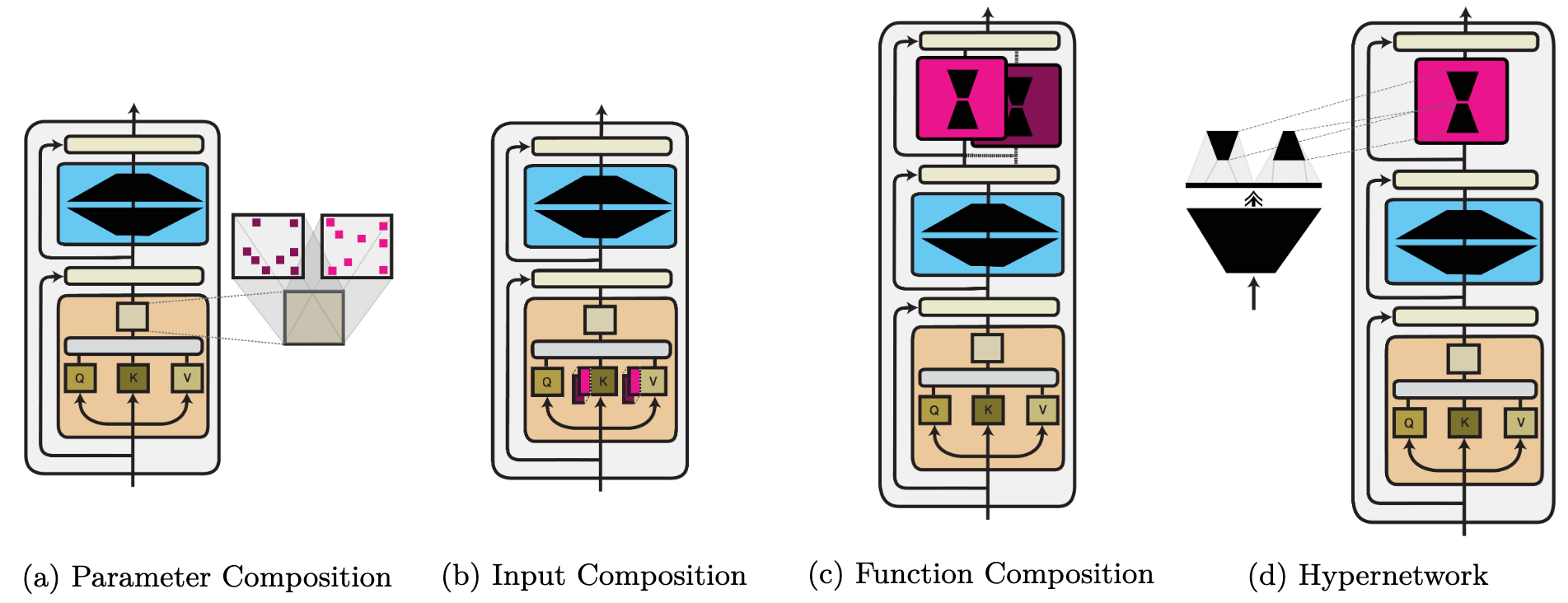
Parameter composition. We identify two main ways modules are used to change the parameters of a model: a) updating a sparse subset of parameters and b) updating parameters in a low-dimensional subspace. Sparse methods are closely related to pruning and the lottery ticket hypothesis. Sparse methods can be structured and only applied to specific parameter groups.
Input composition. Prompt-based learning can be seen as finding a task-specific text prompt whose embedding $\phi$ elicits the desired behaviour. Alternatively, continuous prompts can be learned directly—in the input or at each layer of a model.
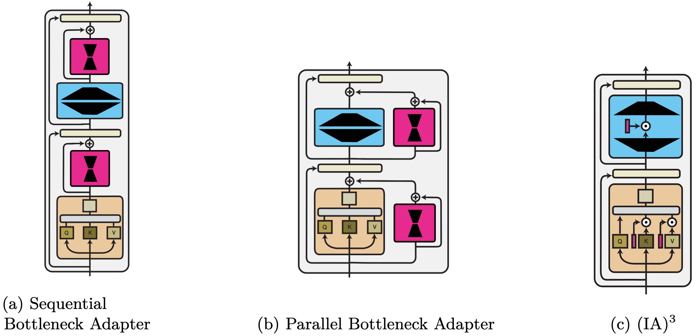
Function composition. This is the most general category. It subsumes standard multi-task learning methods, modules that adapt a pre-trained model (known as 'adapters'), and rescaling methods. In addition, parameter and input composition methods can also be expressed as function composition. For illustration, we provide examples of three function composition methods below.
Module parameter generation. Instead of learning module parameters directly, they can be generated using an auxiliary model (a hypernetwork) conditioned on additional information and metadata.
We provide a high-level overview of some of the trade-offs of the different computation functions below. Refer to the tutorial slides or the survey for detailed explanations.
| Parameter efficiency | Training efficiency | Inference efficiency | Performance | Compositionality | Parameter composition | + | - | ++ | + | + |
|---|---|---|---|---|---|
| Input composition | ++ | -- | -- | - | + |
| Function composition | - | + | - | ++ | + |
Routing Function
A routing function $r(\cdot)$ determines which modules are active based on a given input by assigning a score $\alpha_i$ to each module from an inventory $M$. We give an overview of the different routing methods below.
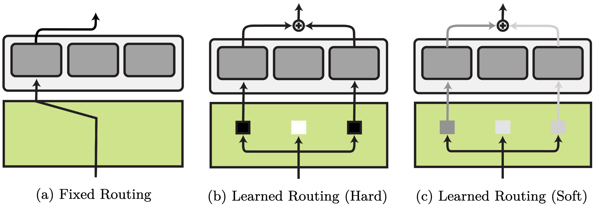
The routing function can be fixed and each routing decision is made based on prior knowledge about the task. Alternatively, routing can be learned. Learned routing methods differ in whether they learn a hard, binary selection of modules or a soft selection via a probability distribution over modules.
Fixed routing. Fixed routing employs metadata such as the task identity to make discrete routing decisions before training. Fixed routing is used in most function composition methods such as multi-task learning and adapters. Fixed routing can select different modules for different aspects of the target setting such as task and language in NLP or robot and task in RL, which enables generalisation to unseen scenarios.
Learned routing. Learned routing is typically implemented via an MLP and introduces additional challenges, including training instability, module collapse, and overfitting. Current learned routing methods are often sub-optimal as they under-utilise and under-specialise modules. However, when there is no one-to-one mapping between task and corresponding skill, they are the only option available.
Hard learned routing. Hard learned routing models the choice of whether a module is active as a binary decision. As discrete decisions cannot be learned directly with gradient descent, methods learn hard routing via reinforcement learning, evolutionary algorithms, or stochastic re-parametrisation.
Soft learned routing. Soft routing methods sidestep a discrete selection of modules by learning a weighted combination in the form of a probability distribution over available modules. A classic example is mixture of experts. As activating all modules is expensive, recent methods learn to only route the top-$k$ and even top-1 modules. Routing on the token level leads to more efficient training but limits the expressiveness of modular representations.
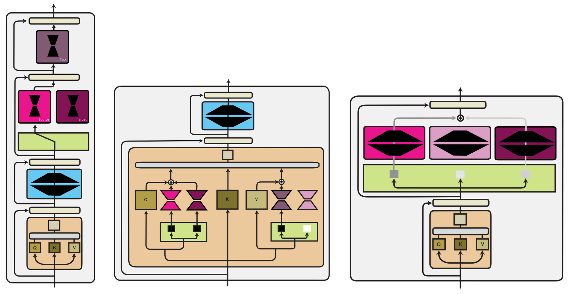
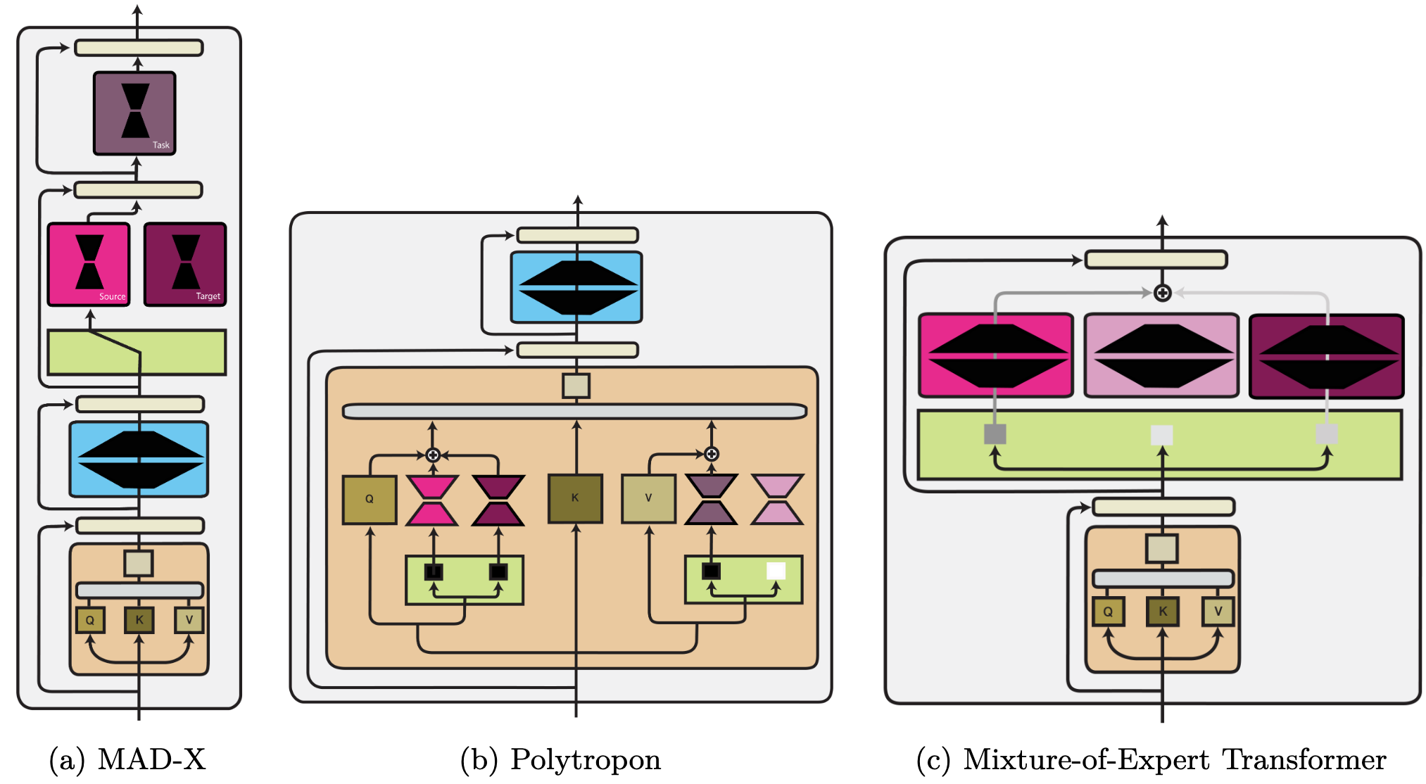
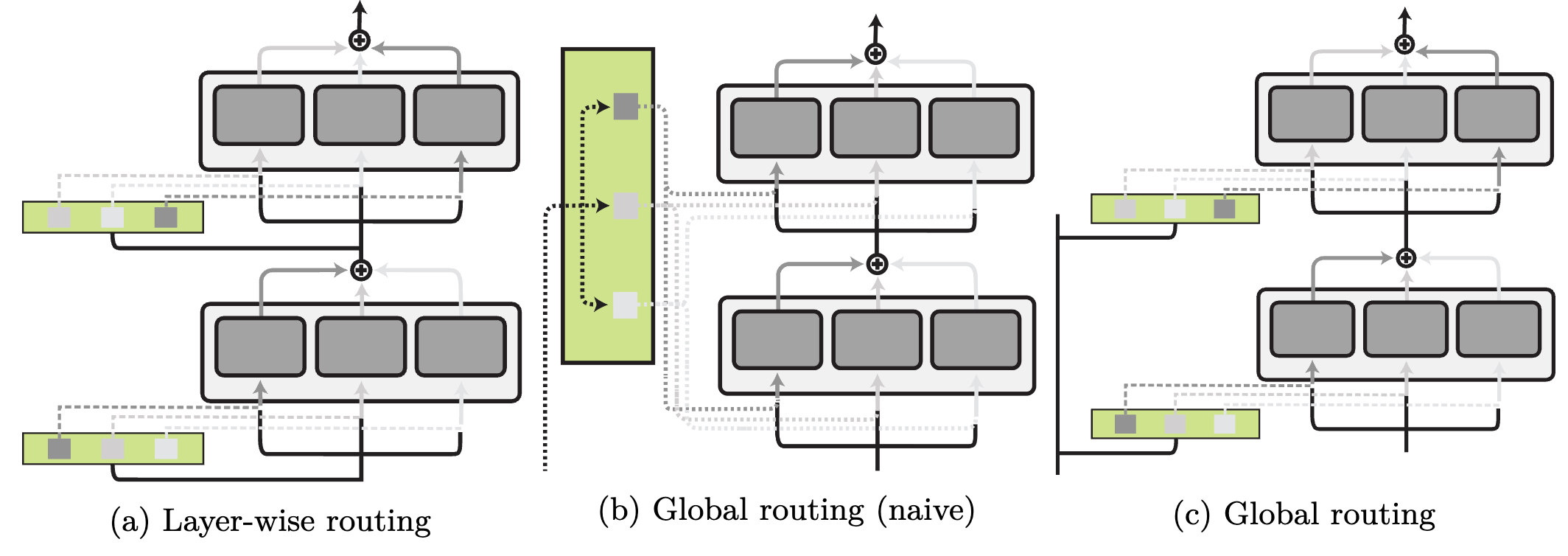
Level of routing. Routing can select modules globally for the entire network, make different allocations per layer, or even make hierarchical routing decisions. We illustrate different routing levels below.
Aggregation Function
The aggregation function determines how the outputs of modules selected via routing are combined. In practice, routing and aggregation are often combined. Aggregation functions can be categorised similarly to computation functions; whereas computation functions compose shared model parts with module components, aggregation functions aggregate multiple module components on different levels:
- Parameter aggregation. Module parameters are aggregated: $f_i^\prime(\boldsymbol{x}) = f_{\boldsymbol{\phi_i}^{1} \oplus \dots \oplus \boldsymbol{\phi}_i^{|M|}}(\boldsymbol{x})$.
- Representation aggregation. Modular representations are aggregated: $f_i^\prime(\boldsymbol{x}) = f_{\boldsymbol{\theta}_i}(\boldsymbol{x}) \oplus f_{\boldsymbol{\phi}_i^1}(\boldsymbol{x}) \oplus \dots \oplus f_{\boldsymbol{\phi}_i^{|M|}}(\boldsymbol{x})$.
- Input aggregation. Module parameters are concatenated at the input level: $f_i^\prime(\boldsymbol{x}) = f_{\boldsymbol{\theta_i}}([\boldsymbol{\phi_i^1}, \dots, \boldsymbol{\phi_i^{|M|}}, \boldsymbol{x}])$.
- Function aggregation. Modular functions are aggregated: $f_i^\prime(\boldsymbol{x}) = f_{\boldsymbol{\phi}_i^{1}} \circ ... \circ f_{\boldsymbol{\phi}_i^{|M|}}(\boldsymbol{x})$.
Parameter aggregation. Aggregating information from multiple modules by interpolating their weights is closely linked to linear mode connectivity, which shows that under certain conditions such as the same initialisation, two networks are connected by a linear path of non-increasing error. Based on this assumption, modular edits can be performed on a model using arithmetic operations in order to remove or elicit certain information in the model.
Representation aggregation. Alternatively, the outputs of different modules can be interpolated by aggregating the modules' hidden representations. One way to perform this aggregation is to learn a weighted sum of representations, similar to how routing learns a score $\alpha_i$ per module. We can also learn a weighting that takes into account the hidden representations, such as via attention.
Input aggregation. In prompting, providing a model with multiple instructions or multiple exemplars via concatenation can be seen as a form of input aggregation. Soft prompts can be learned for different settings such as task and language or attributes and objects and aggregated via concatenation.
Function aggregation. Finally, we can aggregate modules on the function level by varying the order of computation. We can aggregate them sequentially where the output of one module is the input of the next module, etc. For more complex module configurations, we can aggregate modules hierarchically based on a tree structure.
Training Setting
The last dimension along which we can differentiate modular methods is the way they are trained. We identify three modular training strategies: 1) joint training; 2) continual learning, and 3) post-hoc adaptation.
Joint training. In multi-task learning settings, modular task-specific components are trained jointly to mitigate catastrophic interference, with fixed or learned routing. Joint training can also provide a useful initialisation for modular parameters and allow for the additional of modular components in later stages.
Continual learning. During continual learning, new modules are introduced into the model over time. The parameters of previous modules are typically frozen while new modules are connected to existing modules in different ways.
Post-hoc adaptation. These methods are also known as parameter-efficient fine-tuning as they are typically used to adapt a large pre-trained model to a target setting. We cover such methods for NLP in our EMNLP 2022 tutorial.
Purposes of Modularity
Many of the above methods are evaluated based on their ability to scale large models or enable few-shot transfer. Modularity is also crucial for other applications involving planning and systematic generalisation, including 1) hierarchical reinforcement learning; 2) neural programme induction; and 3) neural causal inference. We illustrate them below.
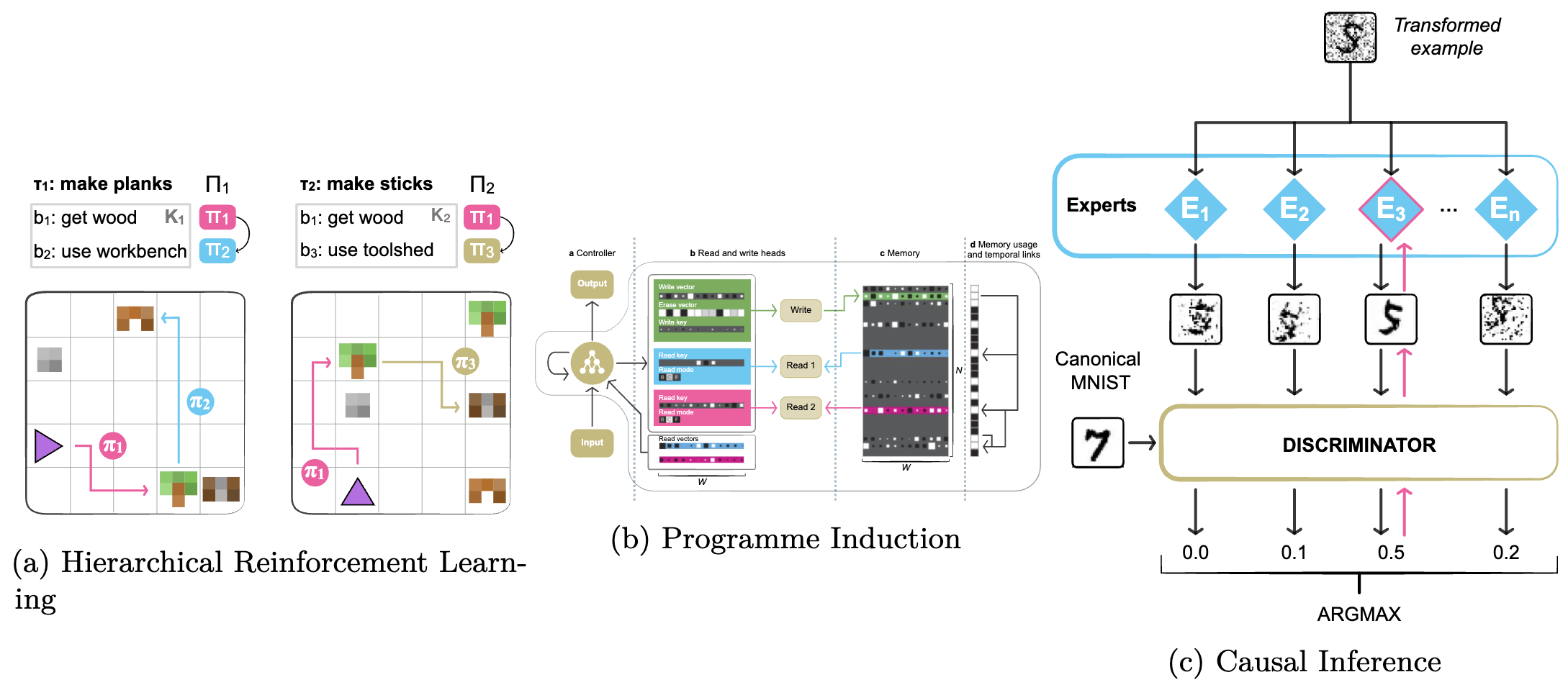
Hierarchical reinforcement learning. In order to learn over large time spans or with very sparse and delayed rewards in RL, it is often useful to learn intermediate abstractions, known as options or skills, in the form of transferable sub-policies. Learning sub-policies introduces challenges related to specialisation and supervision and the space of actions and options. Strategies used to address them involve intrinsic rewards, sub-goals, and language as an intermediate space.
Programme simulation. Modularity can also be used to simulate programmes by constructing a programme graph dynamically based on an input or globally based on a task description. In addition to routing and computation functions, such architectures can be extended with an external memory. Programme simulation is useful when tasks rely on performing the correct sequence of sub-tasks.
Causal inference. Modularity in causal inference methods reflects the modularity in the (physical) mechanisms of the world. As modules are assumed to be independent and reusable, ML models mirroring this structure are more robust to interventions and local distribution shifts. Challenges include specialising each module towards a specific mechanism as well as jointly learning abstract representations and their interaction in a causal graph.
Applications in Transfer Learning
The presented methods are used in a variety of applications. We first highlight common applications in NLP and then draw analogies to applications in speech, computer vision, and other areas of machine learning.
Machine translation. In MT, bilingual adapters have been used to adapt a massively multilingual NMT model to a specific source–target translation direction. Such work has been extended to more efficient monolingual adapters. Hypernetworks have been used to enable positive transfer between languages. Other approaches such as language and domain-specific subnetworks and mixture-of-experts have also been applied.
Cross-lingual transfer. Language modules are combined with task modules to enable transfer of large models fine-tuned on a task in a source language to a different target language. Within this framework, many variations have been proposed that learn adapters for language pairs or language families, learn language and task subnetworks, or use a hypernetwork for the generation of various components.
Domain adaptation. Domain-specific modular representations have been learned using adapters or subnetworks. A common design is to employ a set of shared modules and domain modules that are learned jointly, with additional regularisation or loss terms on the module parameters.
Knowledge injection. Modules can also be used to store and inject external knowledge, which can be combined with language, domain, or task knowledge. A common strategy is to train modules on synthetic data created based on the information in a knowledge base.
Speech processing. In speech, similar methods have been explored as in NLP. The main differences are that the underlying model is typically a wav2vec variant and modular representations are optimised based on the CTC objective. The most common setting is to learn adapters for ASR.
Computer vision and cross-modal learning. In computer vision, common module choices are adapters and subnetworks based on ResNet or Vision Transformer models. For multi-modal learning, task and modality information are captured in separate modules for different applications. The recent Flamingo model, for instance, uses frozen pretrained vision and language models and learns new adapter layers to condition the language representations on visual inputs.
Future Directions
Future directions include combining different computation functions, gaining a better understanding of the nature and differences of different modular representations, integrating learned routing in pre-training, benchmarking routing methods, composing subnetwork information directly, developing learned aggregation methods, and creating extensible modular multi-task models, among others.
Conclusion
We have presented a categorisation of modularity in deep learning across four core dimensions. Given the trend of pre-training larger and larger models, we believe modularity will be crucial. It will enable more sustainable model development by modularising parts and developing modular methods that address current limitations and can be shared across different architectures. But modularity may also facilitate a shift away from a concentration of model development in a few institutions and to distributing the development of modular components across the community.
Citation
For attribution in academic contexts or books, please cite our survey as:
Jonas Pfeiffer and Sebastian Ruder and Ivan Vulić and Edoardo M. Ponti, "Modular Deep Learning". arXiv preprint arXiv:2302.11529, 2023.
BibTeX citation
@article{pfeiffer2023modulardeeplearning,
    author = {Pfeiffer, Jonas and Ruder, Sebastian and Vuli{'c}, Ivan and Ponti, Edoardo M.},
    title = {{Modular Deep Learning}},
    year = {2023},
    journal = {CoRR},
    volume = {abs/2302.11529},
    url = {https://arxiv.org/abs/2302.11529},
}
Please cite our tutorial as:
Sebastian Ruder and Jonas Pfeiffer and Ivan Vulić. "Modular and Parameter-Efficient Fine-Tuning for {NLP} Models". Proceedings of the 2022 Conference on Empirical Methods in Natural Language Processing: Tutorial Abstracts, 2022.
BibTeX citation:
@inproceedings{ruder-etal-2022-modular,
    title = "Modular and Parameter-Efficient Fine-Tuning for {NLP} Models",
    author = "Ruder, Sebastian  and
      Pfeiffer, Jonas  and
      Vuli{\'c}, Ivan",
    booktitle = "Proceedings of the 2022 Conference on Empirical Methods in Natural Language Processing: Tutorial Abstracts",
    month = dec,
    year = "2022",
    address = "Abu Dubai, UAE",
    publisher = "Association for Computational Linguistics",
    url = "https://aclanthology.org/2022.emnlp-tutorials.5",
    pages = "23--29",
}